Requirements for this tutorial:
- Python
- NumPy
- Pandas
- Sci-kit Learn (sklearn)
Post Summary: This tutorial covers the topic of Linear Regression (LR) using gradient descent. It’s a simple and very widely understood machine learning algorithm. This tutorial will walk through an implementation of LR from scratch written in Python. LR is a simple example of a supervised machine learning technique. Supervised learning is a branch of machine learning that learns from labelled data with known true values.
Note: While I'm in the process of setting up a comments section on the tutorial/blog pages, please feel free to provide feedback via my email
I just came here for the code:
1. import numpy as np
2. import pandas as pd
3. from sklearn.datasets import load_boston
4. from sklearn.metrics import r2_score
5. import math
6.
7. def train_test_split(x, y, ratio, seed=1):
8. 	    np.random.seed(seed)
9.  	indices = np.random.permutation(len(y))
10. 	index_split = int(np.floor(ratio * len(y)))
11. 	x_train = x.iloc[indices[: index_split]]
12. 	x_test = x.iloc[indices[index_split:]]
13. 	y_train = y.iloc[indices[: index_split]]
14. 	y_test = y.iloc[indices[index_split:]]
15. 	return x_train, x_test, y_train, y_test
16.
17. def add_theta_0(x, X):
18. 	x["INTERCEPT"] = pd.Series(np.ones(X.shape[0]))
19. 	return x
20.
21. r=0.77; s=1; min_error = 10e-10
22. num_iters = 10000; gamma = 0.01
23.
24. boston = load_boston()99
25. boston_dataset = pd.DataFrame(boston.data, columns=boston.feature_names)
26. boston_dataset['MEDV'] =  boston.target
27. y = boston_dataset.MEDV
28. X = boston_dataset.drop(['MEDV'], axis=1)
29.
30. X_train, X_test, y_train, y_test = train_test_split(X, y, r, seed=s)
31. X_train = add_theta_0((X_train - X_train.mean(axis=0))/ X_train.std(axis=0), X)
32. X_test = add_theta_0((X_test - X_test.mean(axis=0))/ X_test.std(axis=0), X)
33.
34. init_weights = np.zeros(len(X_train.columns))
35. weights_list = [init_weights]
36. weights = init_weights
37. losses = []
38. prev = math.inf
39.
40. for n_iter in range(num_iters):
41. 	error = y_train - X_train.dot(weights)
42. 	derivative = -X_train.T.dot(error) / len(error)
43. 	loss = np.sqrt(2 * 1/2*np.mean(error**2))
44. 	weights = weights - gamma * derivative
45. 	weights_list.append(weights)
46. 	losses.append(loss)
47. 	if(abs(loss - prev) < min_error) :
48. 		print("Reached Convergence !")
49. 		break
50. 	prev = loss
51. params = weights_list[-1]
The code above can also be found on my Github.
Section 1: Some Preliminary Theory
LR is a statistical model which observes the linear relationships between a dependent variable y, and a set of independent variables X. In a simple LR model, the aim is to model the data in a manner according to the following equation:
where h_θ is the prediction we make using the input data X, and the weights that are to be learned, θ. X is the independent variable that we have observed and recorded. θ_0 and θ_1 are the weights or coefficients that we want to learn in order to predict h_θ correctly. This is known as a simple linear regression.
Generally, the number of weights we have to learn is equal to the number of
independent variables in X from the dataset we are using, plus one*.
For example, if we input a dataset with 10 columns in the data,
we will have 11 weights that must be learned in order to successfully predict our h_θ value.
* The plus one here refers to θ_0, which doesn’t have a corresponding value in the original observed dataset.
A linear regression model with many independent variables is either known as multiple LR or Polynomial LR. Note that the X’s and θ’s can be written more concisely using linear algebra notation. This will result in:
It is also possible to further simplify the notation here by adding in an extra column to the x matrix and the values will be 1. This extra column will be in place where X_0 should be. This means that we have an X column that corresponds to θ_0, which will result in a more simplified equation:
With some basic knowledge of maths, we know that the weight θ_0 corresponds to the intercept with the y-axis. In
machine learning, this is generally called the bias, due to the fact that it is added to offset all of the predictions
that are made from the x-axis. The remaining θ values correspond to the slope of the line (in however many dimensions
are present in the data).
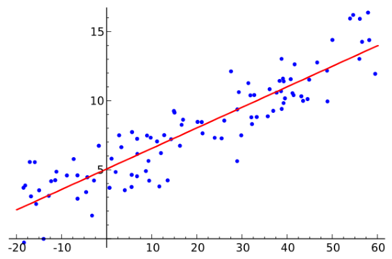
From the above image, we can visually understand what we are trying to achieve with LR: To find the best values for the weights that can be used to estimate the dependent variable y - visually, the learned weights are used to plot the red line and the dependent variable is plotted in blue. In order to learn these weights, we first need to make a prediction. The equation used to make this was described above and called h_θ (x) - The prediction function.
Once we make this prediction however, we don’t necessarily know if it’s any good. It could be spot on and predicting values very accurately, or more likely, its performing very poorly and is predicting at random. To overcome the issue, we need to alter some aspect of the equation discussed above. Since we can’t update the data to fit with our needs, we must therefore update the weights.
The next step required in the LR algorithm is to compute the error, or how far wrong our initial prediction is from the actual y value: Simply put, we are computing the squared difference between the actual dependent variable, y, and our previously predicted value h_θ (x). The reason that we square the error is because we want to know by how much we got it wrong.
By way of analogy, imagine you are playing a game of darts and are training to successfully hit the bulls eye. If you throw a dart and are 1 inch too high, you missed the bulls eye by 1 inch. If you throw the dart again and miss (again) but this time, you hit1 inch too low, you still missed the bulls eye by 1 inch again, regardless of being too high or too low.
There are two reasons as to why we use the squared error. Firstly, using the squared error will force the values to be positive. I’m sure some of you are thinking, ‘well, if all we want to do is to force the error to be positive, we can also use the absolute value!’ which is true. You can. However, there is another reason as to why we use the squared error, which is that large errors are made even larger and small errors are made even smaller. The reason for this, is we don’t need to worry hugely about small errors and we really need to worry about large errors.
As an analogy, consider you are in work one day and you make two mistakes. Firstly, you spilled your morning coffee in the canteen. This is a small mistake and is easily cleaned with a towel. Secondly, since you didn't have your morning coffee, you're tired and groggy - In a sleepy, coffee depraved haze you drop a table in the prod. database. The small error of spilling your coffee is insignificant when compared to dropping a production table in a work database. The big error should be fixed at all costs, while the smaler error can be let go.
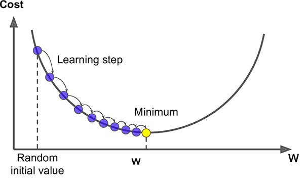
Once we know that we are wrong in our prediction by some value, the next step if to figure out how to minimise this error. Image our error follows the plot below. We can see that the weights start of at the ‘Random initial Value’ and we want to try change the weights that minimises the error; also known as the cost. To do this, we take the derivative of the error function (the mean squared error).
Or if we were computing this over many training samples at a time, the error function would then be:
So, when we take the derivative of this function we obtain:
This now gives us the direction in which we want to go to reduce the error, and know I will introduce a new term called alpha, or the learning rate.
This constant tells us how far we want to move in the direction of the derivative. If alpha is too large, we could actually diverge, while if alpha is too small, it may take a very long time to converge on the desired weights. To mathematically define these operations consider the equation(s) below:
Here, we alter the value of the weights by an amount alpha in the direction of error_deriv which should converge on the minimum value if we have implemented everything correctly.
So, now we know how we want to make our prediction, and we know that we want to find the best values of θ that will keep our error small, and we know we should use gradient descent to find the minimum value of the error/cost function we can now start implementing the above theory as code.
Section 2: Putting Theory into practice:
Now, imagine that you are considering moving to Boston, MA, and you want to purchase a house. If you, for some strange
reason, do not have access to a real estate agent, but have access to a datset relating to the prices of houses in
Boston and you want to know what sort of house fits within your budget, you could use this to estimate the cost of
your new home!
Precautionary disclaimer: Do not use this tutorial as a means of valuating the price of real houses! This tutorial is
simply to illustrate the inner workings of the LR model.
1. # Imports
2. import numpy as np
3. import pandas as pd
4. from sklearn.datasets import load_boston
5. from sklearn.metrics import r2_score
6. import math
7.
8. # required constants for script
9. r=0.77; s=1; min_error = 10e-10
10. num_iters = 10000; gamma = 0.01
11.
12. # Load data
13. boston = load_boston()
14. boston_dataset = pd.DataFrame(boston.data, columns=boston.feature_names)
15. boston_dataset['MEDV'] =  boston.target
16. y = boston_dataset.MEDV
17. X = boston_dataset.drop(['MEDV'], axis=1)
18.
19. # Split data into training and testing sets
20. X_train, X_test, y_train, y_test = train_test_split(X, y, r, seed=s)
21. X_train = add_theta_0((X_train - X_train.mean(axis=0))/ X_train.std(axis=0), X)
22. X_test = add_theta_0((X_test - X_test.mean(axis=0))/ X_test.std(axis=0), X)
23.
24. #### START LINEAR REGRESSION ####
25. # Define variables to store weights and losses
26. init_weights = np.zeros(len(X_train.columns))
27. weights_list = [init_weights]
28. weights = init_weights
29. losses = []
30. prev = math.inf
31.
32. for n_iter in range(num_iters):
33. 	# compute loss, gradient and rmse(actual loss)
34. 	error = y_train - X_train.dot(weights)
35. 	derivative = -X_train.T.dot(err) / len(error)
36. 	loss = np.sqrt(2 * 1/2*np.mean(error**2))
37.
38. 	# gradient w by descent update
39. 	weights = weights - gamma * derivative
40.
41. 	# store w and loss
42. 	weights_list.append(weights)
43. 	losses.append(loss)
44.
45. 	#Stop earlier if we reached convergence
46. 	if(abs(loss - prev) < min_error) :
47. 		print("Reached Convergence !")
48. 		break
49. 	prev = loss
50.
51. #Get final weights
52. params = weights_list[-1]
There were a couple of helper functions that I also implemented to i) split the data into train and test sets, ii) to standardise the data and iii) evaluate the implementation using the R squared measure. The code for these are shown below and arent discussed later since they're only helper functions which can be replicated with the train_test_split method in sklearn:
53. def train_test_split(x, y, ratio, seed=1):
54. 	"""split the dataset based on the split ratio."""
55. 	# set seed to produce reproducable results
56. 	np.random.seed(seed)
57.
58. 	# generate random indices
59. 	indices = np.random.permutation(len(y))
60. 	index_split = int(np.floor(ratio * len(y)))
61.
62. 	# create split
63. 	x_train = x.iloc[indices[: index_split]]
64.	    x_test = x.iloc[indices[index_split:]]
65. 	y_train = y.iloc[indices[: index_split]]
66. 	y_test = y.iloc[indices[index_split:]]
67. 	return x_train, x_test, y_train, y_test
68.
69. def add_theta_0(x, X):
70. 	x["INTERCEPT"] = pd.Series(np.ones(X.shape[0]))
71. 	return x
| Operation | Operation Explained |
|---|---|
| X | Input matrix of independent variables: Each row is a unique training sample |
| y | Output matrix of dependent varables: Each row is unique training sample |
| * | element wise multiplication: Two vectors of equal dimensions are multiplied together to produce a resultant matrix of the same dimension as the two original matrices. |
| - | element wise subtraction: Two vectors of equal dimensions are subtracted frome each other to produce a resultant matrix of the same dimension as the two original matrices |
| x.dot(y) | If x and y are vectors this is the dot product, if both x and y are matrices, this is matrix multiplication and if either or y is a vector or a matrix, this is a vector-matrix multipication |
| add_theta_0 | This is a helper function that was added to append the INTERCEPT column to the independent variables. This is done to simplify the matrix multiplication from y = theta_0 + x*remaining_thetas to y = theta*x |
| R Squared | R Squares is a statistical measure that ranges from 0-100% and is used to illustrate the amount of explained variance in the learned model. The formula for R squared is: R^2 = 1 - explained variation/total variation |
As you can see from the 'R2 after training', we have successfully learnned a series of coeffecients that have produced a relatively high R Squared value, meaning that the learned weights explaining 73.64% of the variation between the predicted and actual dependent variable. Congratulations, you can now use this to predict the price of your new house in Boston.
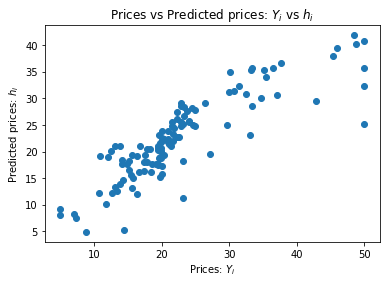
The above plot shows the difference between the actual value of the houses versus the prediction. In an ideal world, the scatter plot that you can see above would show a more linear relationship between the data, thus explaining more of the variance in the data. However, since the model doesn't fit to the data 100%, the scatter plot is not producing a perfect line.
Before I describe the processes involved in the code, I would highly recommend playing with the code above to get an intuitive feeling for how it works: Try changing some of the values to understand how it impacts on the final model, will more or less indepenedent variables improve or disimprove the results obtained above? You should be able to run the code with the helper functions as is.
Now that we have the required theory out of the way, and you have (hopefully) read through the code above, we will
walk through this code chronologically explaining all steps required to estimate our weights.
Note: I would recommend opening two tabs on your screen so you can see the code and the walk through
togetther while you read!
Lines: 2 - 6 These import the required libraries for this code to work.
Lines: 9 & 10 These are the constants which are used as inputs to our functions and algorithms. r is used to define the splitting ratio of our dataset: the training dataset will be 77% of the original dataset and the testing set will therefore be 33%. s is a seed that we input into the numpy's random number generator to ensure that the results obtained here are reproduceable. num_ters defines the maximum number of iterations we calculate for this algorithm. min_error is used for early stopping - if we have learned the weights to be within the range of min_error, we can stop training. alpha is the learning rate - this controls how aggressive our steps are in gradient descent.
Lines: 13 - 17 These lines load the Boston housing data from the sklearn datasets, split the data into the dependent variable and independent variable datasets.
Lines: 20 - 22 Takes the X and y data, splits them into thetraining and testing sub-datasets, standardises the dependent variables, and then finally adds in a new column that corresponds to X_0: a feature that is added only to simplify the maths later.
Lines: 26 - 30Here we are initialising the variables that will be needed during the learning process. They will be used to keep track of the weights we are learning and the losses we generate during training.
Lines: 34 Here, we make a prediction with X_train.dot(weights) (Which corresponds to h_θ (x)) and we compare the result to the actual values in y. This is our error; how wrong our prediction is from the real values.
Lines: 35 We apply the first step required for Gradient Descent, compute the derivative of our cost function. This value will be used later on in updating our weights.
Lines: 36 Here we're computing and keeping track of the Root Mean Square Error (RMSE) - the loss. The current loss value will be compared the previous loss value in oreder to determine if we should stop learning early.
Lines: 39 Here we finally update the weights using gradient descent! We incrementally update the original weights by adding our derivative (or gradient) times the learning rate (alpha) - This moves our weight by an amount alpha in direction of the derivative.
Lines: 42 & 43 These two lines keep track of the previous loss and weight values that we have enountered on this learning process.
Lines: 46 - 48 This is where we can stop early. If the difference between our current and previous loses are negligible, i.e., less then our min_error value, we can stop here since we probably won't update the models much more beyond this point.
That's all well, and good - But how does this actually compare to what's used in industry?
For this, I will simply share the code and results; which again is on my github here. This implementation was done using sklearn.
1. import numpy as np, math, pandas as pd
3. from sklearn.datasets import load_boston
4. from sklearn.metrics import r2_score
5. from sklearn.linear_model import LinearRegression
6. from sklearn.model_selection import train_test_split
7.
8.  boston = load_boston()
9. boston_dataset = pd.DataFrame(boston.data, columns=boston.feature_names)
10. boston_dataset['MEDV'] =  boston.target
11.
12. y = boston_dataset.MEDV
13. X  = boston_dataset.drop(['MEDV'], axis=1)
14.
15. # y = boston.target
16.
17. X_train, X_test, y_train, y_test = train_test_split(X, y, test_size=0.33, random_state=42)
18.
19. reg = LinearRegression().fit(X_train, y_train)
20. print(reg.score(X_test, y_test))
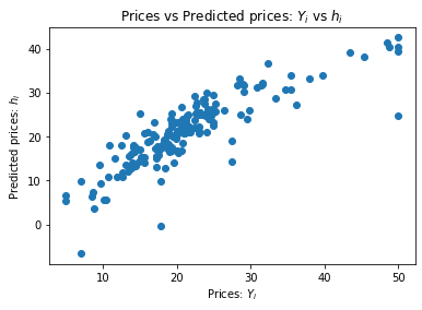
The above plot shows the difference between the actual value of the houses versus the prediction using sklearn.